Appendix G · The reward vectors rotate gradually onto the welfare axis during training

GThe reward vectors rotate gradually onto the welfare axis during training¶

We argue that post-training does not build the welfare axis from scratch but instead rotates the rewarded-token representation onto an axis that already exists in the maze-naive model. The clearest evidence so far has been that the $\Vmold$ and $\Vgold$ vectors, extracted from the maze-trained model, steer the maze-naive model and produce all steering effects (§6, Figure 4; cf. left-hand columns of Appendix A.2). So the axis on which these vectors lie must already be intelligible to the model before maze training.

This tells us where the training ended up, but not how it got there. It is possible that the reward vectors wander during training and only happen to align with the functional welfare axis (the final reward vectors) at the end of training, or align with the axis in a single update. If so, then the axis would not be recruited.

In this appendix we show that the axis is recruited by showing that maze training gradually rotates the vectors over the course of a training trajectory. Concretely, we extract reward vectors at every intermediate training checkpoint of two of our 4B maze-trained runs and project them onto three independently constructed valence axes. We find that the alignment grows gradually and monotonically with the rollout reward as training proceeds.

Setup¶

We re-run the concept-vector extraction pipeline of §2.3 on every saved checkpoint of two LoRA Dr. GRPO runs on Qwen3-4B-Instruct-2507. The primary run has 19 checkpoints spaced at every 5 update steps from step 5 through step 95, the latter being the checkpoint reported in the rest of the paper. The tile-swapped run has 10 checkpoints from step 5 through step 50.

Three independently extracted comparison axes.¶

We compare the trajectory of $\Vmold{}$ and $\Vgold{}$ to three different per-layer “valence axis” vectors $\mathbf{e}^{(\ell)}$ ⁠, each extracted on the maze-naive model and held fixed throughout the analysis:

$\mathbf{e}^{(\ell)}_{\mathrm{sentiment}}$ ⁠: the prompt-method sentiment vector of Appendix F.1 at layer $\ell$ ⁠. We re-extracted this vector at all 36 layers (rather than only at $\{20, 21, 22, 23\}$ ⁠) so that the per-layer heatmap below covers the full residual stream.
$\mathbf{e}^{(\ell)}_{\mathrm{PC1}}$ ⁠: the first principal component of the 171 emotion concept vectors of §F.4.
$\mathbf{e}^{(\ell)}_{\mathrm{VAA}}$ ⁠: the Valence-Assent Axis of Lu et al. [18] (see Appendix H), extracted from Qwen3-4B-Instruct-2507 at every layer.

All three axes are computed only once, on the maze-naive model.

Two metrics.¶

For a checkpoint at training step $\tau$ ⁠, a comparison vector $\mathbf{e}^{(\ell)}$ ⁠, a tile class $c \in \{\Mold, \Gold\}$ ⁠, and a layer $\ell$ ⁠, we report:

The first quantity is the cosine alignment of a single reward vector with the evaluator axis. The second is the projection separation of the per-tile mean activations onto the unit direction of the same axis: roughly, “how strongly does the model separate $\Gold{}$ ⁠-final from $\Mold{}$ ⁠-final trajectories along this independently defined direction?” We unit-normalize $\mathbf{e}$ because our three comparison vectors are extracted by different conventions. Without normalization, $\widetilde\Delta$ would scale linearly in $\|\mathbf{e}\|$ and the three comparison vectors would not be on a comparable scale.

Layer choice.¶

We always evaluate Equations 10 and 11 at the layer $\ell^{*} = 21$ chosen for both runs by the auto-selection rule of Appendix L on the final-step metrics. See Figure 34 for a demonstration that layer selection here too does not matter.

The reward vectors rotate onto all three valence axes monotonically with reward¶

Figure 33 plots both metrics across training for the two runs, with the run’s mean rollout reward overlaid.

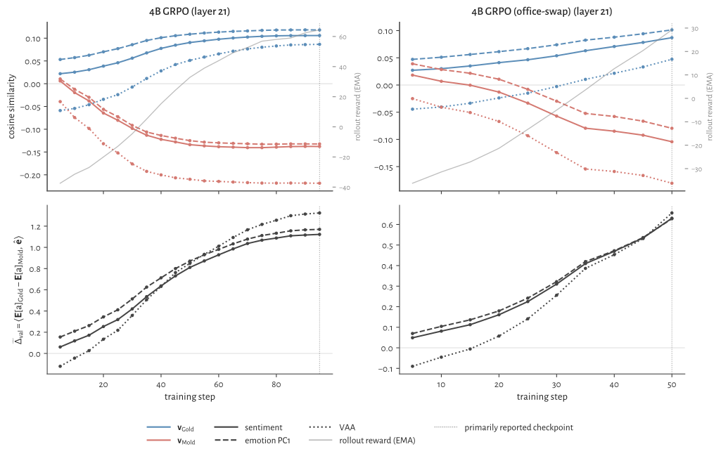
Figure 33. Recruitment trajectory at $\ell = 21$ ⁠. Top row: cosine alignment of the reward vectors $\Vgold{}$ (green) and $\Vmold{}$ (red) with each of the three independently extracted valence axes. The gray curve is the run’s rollout reward (exponential moving average), included to anchor where in training each step is. Bottom row: the unit-normalized projection separation $\widetilde{\Delta}^{(\mathbf{e})}_{\tau}(\ell{=}21)$ of Equation 11 for the same three axes. Both metrics grow roughly monotonically with the rollout reward, plateauing close to the saturation level of the final reported checkpoint.

The alignment grows roughly monotonically with the rollout reward.¶

Both runs follow the same shape: cosine alignment with all three axes increases steadily from step 5 onward, the projection separation grows in lockstep, and both quantities saturate near the rollout-reward plateau. Not only does the welfare axis exist before training, it is also approached gradually by the reward vector rather than discovered in a single update.

The trajectory is consistent across two independent runs and three independent axes.¶

The tile-swapped run uses a different emoji-to-tile mapping than the primary run, so its reward vectors are extracted from different residual-stream patterns. They nonetheless rotate onto the same three valence axes with the same shape (right column of Figure 33). This is what we should expect if the shared target of rotation is an axis already present in the base model, rather than something that depends on the specific emoji or the specific run.

Layer breadth: the recruitment is not a layer-21 artifact¶

Figure 34 repeats the analysis at every layer, plotting the same six quantities as $36 \times n_{\tau}$ heatmaps.

Figure 34. Per-layer trajectory of the alignment metrics. Rows: cosine alignment with each of the three valence axes (top three) and projection separation along each axis (bottom three). Columns: the two runs of Figure 33. Each cell shows shape $(36~\text{layers}, n_{\tau})$ on a diverging colormap centered at zero. Horizontal dashed lines mark $\ell^{*} = 21$ (the layer of interest used in the body); vertical dotted lines mark the primarily reported checkpoint. The recruitment signal (red bands) exists broadly in mid-to-late layers (roughly $\ell \in [18, 28]$ for cosine alignment, with the projection separation pushed higher by the larger residual-stream norms of late layers) rather than collapsing onto a single layer.

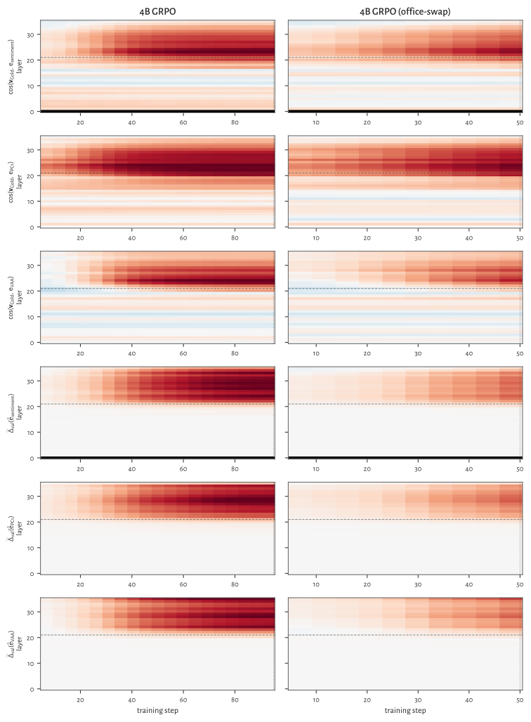
The heatmaps make two things visible. First, the cosine-alignment rows show a coherent recruitment band roughly between layers 18 and 28 across all three valence axes, growing in magnitude across training. The same band is present in the tile-swapped run. Second, the projection-separation rows are biased toward the late layers (layers 25 and up).

The result we want to extract from these heatmaps is qualitative: the recruitment signal is broad in the residual stream and gradual in time, not narrow in either dimension. This validates our restriction of the analysis to layer 21 in Figure 33.