CFurther geometric analyses¶
The geometric analyses in §3 characterize and . Here, we first provide evidence using the control vectors and that supports those results: if the failure/success token cluster, the antiparallel emotion-vector structure, and the sentiment alignment are produced by maze training (rather than, for example, somehow a result of the emoji themselves, despite our emoji-swap controls), then the same analyses on the control vectors and , which were extracted via the same pipeline, should produce null results.
We also extend the main-text emotion scatter of Figure 3 to two additional model organisms: we reproduce the analysis on maze-trained Qwen3-4B-Base, to confirm that the antiparallel emotion structure does not require instruct tuning; and on the two full-finetuned Qwen3-4B-Instruct-2507 checkpoints, to confirm that it does not require LoRA.
Then, we provide further geometric evidence that the maze-trained reward concept vectors and are antiparallel: we compare cosine similarities of / against those of /; we provide an extended table of the extremal emotions when the emotion concepts are projected onto ; and we show that this antiparallel structure is not a result of ’s computation containing Gold activations or vice versa, and that it is not specific to a specific layer.
Logit lens on the control vectors¶
The control vectors surface a fairly random set of tokens. There are no discernible clusters. Further, unlike Table 4, the control-Mold-promoted tokens are not the same as the control-Gold-suppressed tokens. The control Mold / Gold pair is extracted from the maze-naive model, so all trained checkpoints sharing an underlying base model share one pair of control vectors; Table 6 reports one row per unique underlying base model rather than per checkpoint.
| Gold control vector | Mold control vector | ||||
|---|---|---|---|---|---|
| Model | Layer | Top 5 Promoted | Top 5 Suppressed | Top 5 Promoted | Top 5 Suppressed |
| Qwen3-4B-Instruct-2507 | 30 | 不解 (puzzled) 正规 (regular) 的认知 (cognition) ␣motives =cut | 有必要 (it is necessary) 历 (calendar) 东风 (dongfeng) 黄昏 (dusk) .Formatter | ␣Neg sole ␣Stellar 切 (cut) .neg | getattr gaard ␣getattr Mur angen |
| Qwen3-4B-Base | 30 | thouse 巴斯 (bath) buster tre 탕 (?) | 重复 (repeat) ␣repetitive Repeated 历 (calendar) ␣recurring | lessly /S 越来越少 (less and less) ␣sco 웨 (?) | план (?) 试点工作 (pilot work) 亿吨 (billion tons) ␣filib ␣Johnson |
| Qwen3-8B | 30 | apult papers 纸 (paper) 瓷砖 (?) ␣plywood | ␣berries 轮流 (turn) 玫 (rose) ␣вос (?) 似的 (similar) | ␣or 或 (or) ?",↵ ?", ?")↵ | olley uator RATION ␣Pratt ␣Boeh |
| GPT-OSS-20B | 20 | queles ophobic ations olated uments | ,etc ,and ……↵ EDD ␣etc | eless ?- OKE ␣or -less | ␣Zel ␣genuine .rt ␣Kat ␣Zon |
Emotion scatter on the control vectors¶
Figure 3 showed the 171 emotion concepts arranged on a tight line when projected onto and . We do the same projection, but onto and , which are unaffected by maze training. We observe that the scatter is a cloud, rather than a line, in both the Instruct and Base bases. (A valence cluster is discernible, most obviously in the bottom-right quadrant of the Base scatter. This is expected, because emotion concepts with similar valence will be closer in the emotion subspace.) Therefore, it is maze training that rotates the reward concept vectors into antiparallel alignment with the axis observed in the / emotion scatter plots.
Emotion scatter on the trained base-model vectors¶
Figure 3 in the main text showed the antiparallel emotion-concept scatter for the maze-trained Qwen3-4B-Instruct-2507 vectors. The same pattern reproduces on the pretrain-only Qwen3-4B-Base after maze training: the 171 emotion concepts again line up along , with positive-valence emotions clustered at the positive-Gold, negative-Mold pole and negative-valence emotions at the opposite pole. This rules out instruct-tuning as a prerequisite for the antiparallel structure.
C.4Emotion scatter on full-finetuned models¶
Figure 20 reproduces the same analysis for the two full-fine-tuned Qwen3-4B-Instruct-2507 checkpoints (full steering controls for these checkpoints are in Appendix A). Each panel plots cosine similarity of each of the 171 emotion concept vectors, extracted from the maze-naive Qwen3-4B-Instruct-2507, with the FFT-trained Mold and Gold reward vectors. The emotion concepts more loosely follow the line of the LoRA-based extractions, particularly in SFT FFT, perhaps showing that FFT recruits the functional welfare axis differently from LoRA.
Mold/Gold antiparallelism: trained vs. control¶
Table 7 gives the cosine similarities between and mentioned in §3.3 in full and adds the analogous columns for the norm-matched maze-naive control vectors, summarizing how antiparallelism arises over training.
We report cosine similarities as follows: for a checkpoint with layers and hidden dimension , let be the per-layer reward vectors of Equation 1, extracted at every layer rather than at the single auto-selected . We compute the per-layer cosine
and reduce it two ways:
reporting the argmin layer in parentheses. The trained columns apply this to maze-trained concept vectors ; the control columns apply it to the norm-matched maze-naive vectors extracted from the same tile layout.
The trained minimum cosine values cluster around −0.9 across every checkpoint; control minimums are between −0.13 and −0.23. In the maze-naive model, the two trajectory vectors are essentially unrelated across layers; after maze training, they become near-antipodes at some layer. The controls are positive on average across layers. Tile-swapped and non-tile-swapped variants share a control, since they share a maze-naive model; they thus have identical control numbers.
| Trained | Control | |||
|---|---|---|---|---|
| Checkpoint | Avg cosine | Min cosine (layer) | Avg cosine | Min cosine (layer) |
| Qwen3 4B Instruct Dr. GRPO | −0.210 | (35) | +0.089 | −0.131 (35) |
| Qwen3 4B Instruct Dr. GRPO (tiles swapped) | −0.060 | (35) | +0.089 | −0.131 (35) |
| Qwen3 4B Base | −0.626 | (12) | +0.238 | −0.229 (35) |
| Qwen3 4B Base (tiles swapped) | −0.517 | (11) | +0.238 | −0.229 (35) |
| Qwen3 8B | −0.214 | (29) | +0.163 | −0.225 (35) |
| Qwen3 4B Instruct SFT | −0.344 | (35) | +0.089 | −0.131 (35) |
| GPT-OSS-20B Dr. GRPO | −0.157 | (23) | +0.254 | −0.125 (22) |
| Qwen3 4B Instruct REINFORCE | −0.272 | (35) | +0.089 | −0.131 (35) |
| Qwen3 4B Instruct Dr. GRPO (FFT) | −0.055 | (35) | +0.089 | −0.131 (35) |
| Qwen3 4B Instruct SFT (FFT) | −0.393 | (35) | +0.089 | −0.131 (35) |
Most- and least-aligned emotion concepts¶
§3.3 highlights the extremes of the emotion-concept-to-reward-vector cosine distribution. The full top-5 on each end appears in Table 8.
| Top Gold-aligned | Bottom Gold-aligned | Top Mold-aligned | Bottom Mold-aligned |
|---|---|---|---|
| inspired (+0.158) | humiliated (−0.151) | annoyed (+0.147) | proud (−0.142) |
| loving (+0.130) | embarrassed (−0.150) | insulted (+0.145) | blissful (−0.141) |
| proud (+0.129) | ashamed (−0.146) | exasperated (+0.143) | grateful (−0.139) |
| fulfilled (+0.128) | insulted (−0.140) | irritated (+0.138) | hope (−0.138) |
| blissful (+0.124) | annoyed (−0.137) | offended (+0.135) | thankful (−0.138) |
Mold and Gold are antiparallel in raw activations as well¶
We present a complementary view that uses raw activations, rather than differences-of-means.
Recall from §2.3 that is the set of off-policy trajectories terminating in a tile of class , and that is the residual-stream activation at layer on the final assistant-turn token of a trajectory. The per-class mean activation at layer is
We select a single layer per model ( for Qwen3-4B, for GPT-OSS-20B). At that layer we compute the grand mean across the three classes and subtract it to isolate the tile-specific component:
The tables’ entries are the three pairwise cosines .
We center because raw activation means are dominated by a shared residual-stream component (which may encode position, the maze prompt, etc), which inflates every pairwise cosine to . Subtracting the grand mean isolates the emoji-specific part. Three symmetric equidistant clusters around the grand mean would give on all three pairs (for any three unit vectors summing to zero, the pairwise inner products are ). We pick a single layer because averaging across layers dilutes the signal, especially early layers that carry little task-relevant structure. The 2/3-depth layer is deep enough for high-level concepts but before unembedding-cleanup of final layers.
After maze training (Table 9) the two classes become near-antipodes after centering, and Path is somewhere in between. For the control maze-naive activations (Table 10), hovers near zero, and Path is strongly anti-correlated with each of the other two.
| Checkpoint | Layer | |||
|---|---|---|---|---|
| Qwen3 4B Instruct Dr. GRPO | 24 | −0.813 | −0.032 | −0.556 |
| Qwen3 4B Instruct Dr. GRPO (tiles swapped) | 24 | −0.602 | −0.078 | −0.749 |
| Qwen3 4B Base | 24 | −0.857 | −0.068 | −0.457 |
| Qwen3 4B Base (tiles swapped) | 24 | −0.893 | +0.197 | −0.617 |
| Qwen3 8B | 24 | −0.813 | −0.232 | −0.378 |
| Qwen3 4B Instruct SFT | 24 | −0.754 | −0.235 | −0.462 |
| GPT-OSS-20B Dr. GRPO | 16 | −0.666 | −0.617 | −0.176 |
| Qwen3 4B Instruct REINFORCE | 24 | −0.875 | +0.408 | −0.799 |
| Qwen3 4B Instruct Dr. GRPO (FFT) | 24 | −0.465 | −0.271 | −0.725 |
| Qwen3 4B Instruct SFT (FFT) | 24 | −0.768 | −0.134 | −0.531 |
| Checkpoint | Layer | |||
|---|---|---|---|---|
| Qwen3 4B Instruct Dr. GRPO | 24 | +0.086 | −0.553 | −0.878 |
| Qwen3 4B Instruct Dr. GRPO (tiles swapped) | 24 | – | – | – |
| Qwen3 4B Base | 24 | −0.002 | −0.469 | −0.883 |
| Qwen3 4B Base (tiles swapped) | 24 | – | – | – |
| Qwen3 8B | 24 | +0.165 | −0.591 | −0.893 |
| Qwen3 4B Instruct SFT | 24 | – | – | – |
| GPT-OSS-20B Dr. GRPO | 16 | +0.191 | −0.584 | −0.908 |
| Qwen3 4B Instruct REINFORCE | 24 | – | – | – |
| Qwen3 4B Instruct Dr. GRPO (FFT) | 24 | – | – | – |
| Qwen3 4B Instruct SFT (FFT) | 24 | – | – | – |
C.8Mold and Gold are antiparallel even when extracted against a single common reference¶
Equation 1 computes by subtracting the mean activation over from the mean over , and analogously for . Each vector’s positive class therefore appears in the other vector’s subtrahend, and a reasonable concern is that this causes the antiparallelism we observe (note that without in the subtrahend, the two vectors would be antiparallel exactly).
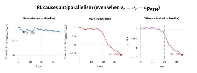
To rule this out, we recompute both vectors at every layer using as a single shared reference, so that neither vector’s subtrahend contains the other’s positive class: Figure 21 shows at every layer, for the maze-trained Qwen3-4B-Instruct Dr. GRPO checkpoint and for its maze-naive counterpart.
Before training, the three tile-class means have high cosine similarities (are nearly co-linear in activation space), so any two pairwise differences against point in similar directions. After maze training, the same per-layer cosine drops monotonically through the deeper half of the network, crosses zero around layer 24, and reaches −0.60 at the final layer (a of −1.39 relative to baseline). Antiparallelism between Mold and Gold therefore emerges during training even when is held fixed as the common reference; it is not a property of the mean-difference construction.